Begin with the plugin
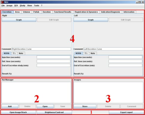
I) Open Image/Stack:
Click on this button to open a single image or a stack. Then choose the image you want to open. A window showing the application is working is displayed. Then, a window appears to choose different options.
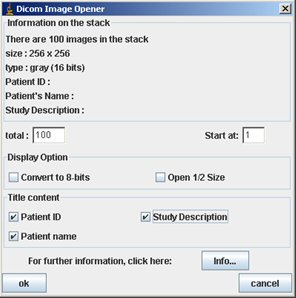
We recommend you to check all the “Title content” and click OK. Then the image/stack appears. Be careful, you can open only one stack/image. You will had to close the opened one to open another stack/image.
II) Brightness/Contrast:
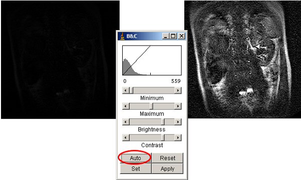
This button opens a window that allows the user to modify the Brightness and Contrast of the image stack. This window is an ImageJ window.
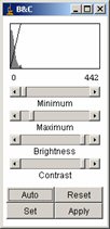
First click on the “Auto” button. The result is usually good.
 III) Export report:
Click on this button to edit a report with all data (curve, computed data, DICOM data, images, …) in PDF format.
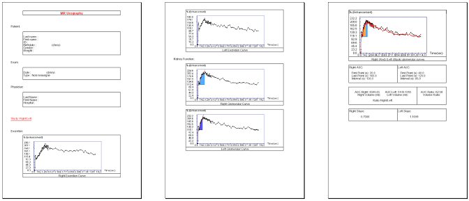
Note that only the tabs present in the interface are saved in the report (cf. Interface configuration).
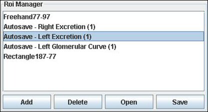
It’s the part of the application where you can view the different ROI you made. When you make an action using a ROI, this one will be saved automatically.
You can add ROI too by your own, save to disk and re-open it. You can select a ROI to display it on the image and work. When you add a ROI manually, you have to choose a name and then to validate it.
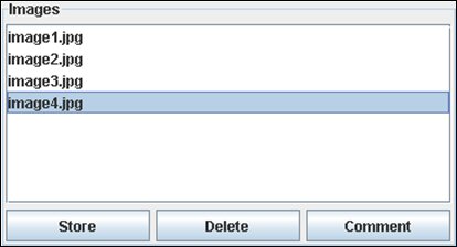
To add images to the report, just click on the “add” button in the images manager. For the first image, you will have to choose a directory where all the data will be saved.
Then you got to add a comment to the image for the report. You can modify the comment by clicking on the “comment” button to change it.
If you want to view a saved image, double click on it in the list.
The different working tools
You can make different assessment with the plugin. Here is the tab bar which allows you to choose your task. We will describe how to make the different works.
 I) Information tab:
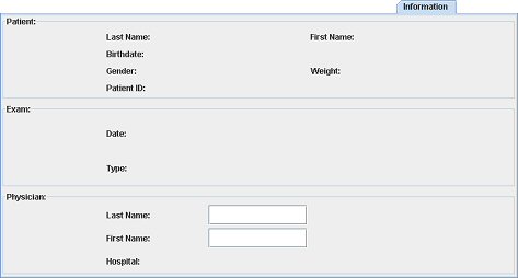
When you open DICOM images, the different fields of this tab are set with the DICOM values. At this step, you can only add the physician last and first name.
II) Indication/Diagnosis tab:
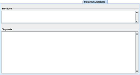
Two fields are displayed: the first one to indicate the indication of the examination and the second one to write the diagnosis you made.
III) Registration & Dynamics tab:
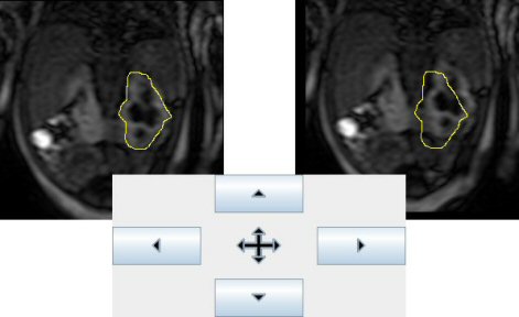
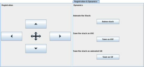 - Registration: Due to breathing, the kidney can move from one image to another. With this tool you can move each image of the stack in order to place correctly the ROI on the kidney.
- Dynamics: You can animate the stack (loop) or save it either as AVI or as animated gif.
�IV) Duration tab:
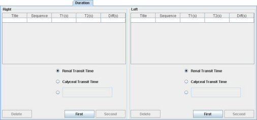
You can compute the time difference between two images. Select the first image in the stack then click the button “First Image”. Do the same thing with the second one and you will get the duration.
Time denominations are already set up for renal transit time and calyceal transit time. However, any time interval between 2 images can be measured. Be careful, once the first image is selected, you must choose the second one on the same sequence.
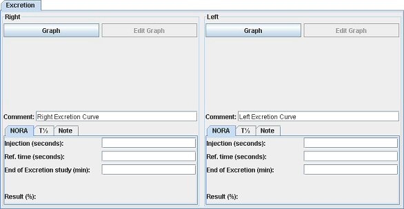
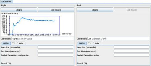
V) Excretion tab:
You can process the excretion assessment in three different ways. The first one is by observing the excretion curves and the others are the NORA and T˝ studies.
1) The graph study:
The goal is to obtain the excretion curve for each kidney or/and pole.
To process the excretion assessment, you have to open a dynamic stack.
The ROI can surround either the entire kidney (or pole) or be limited to the excretory system.
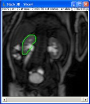
Then click on the “Graph” button. The result is a new window showing the “Excretion curve” (dynamic analysis of the ROI signal intensity).
Be careful:
This curve is normalized according to (Si-So)/So
Si: Signal intensity for any point
So: Averaged signal intensity of the two first points of the curve
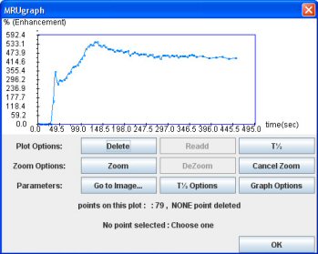
Then, click on “OK”. The curve appears on the main interface.
2) Nora assessment:
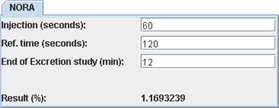
NORA is the normalized residual activity (1) and is defined as the ratio between the signal intensity at a given moment (End of Excretion study) and the renal signal at a reference time (“Ref. time ‘, generally between 1 and 2 minutes). This ratio is derived from nuclear renography and has not been studied in MR. It has to be considered as a research tool. To get the NORA number, you have to look at the previous excretion curve. Then just enter the different parameters for the study and the results will be automatically yielded.
1. Piepsz A, Kuyvenhoven JD, Tondeur M, Ham H. Normalized residual activity: usual values and robustness of the method. J Nucl Med 2002; 43:33-38.
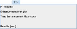
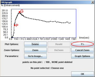
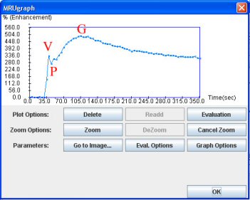
3) T˝ assessment:
As before, you need the excretion curve to process this study.
In the graph window, click the “T˝” button. And then click on the P point (just after the peak) and the maximum point (G).
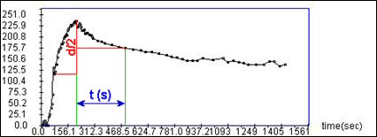
You can see on the next page, what is exactly the value of T˝. It is the time needed by the kidney to eliminate half of the contrast product, considering the baseline as the through after the vascular peak. Like NORA, T1/2 has to be considered like a research tool.
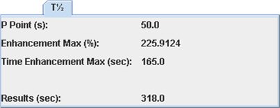
The result appears automatically on the T˝ tab.
VI) Split Renal Function (Area tab, Volume tab and Area & Volume tab):
The goal is now to evaluate the percentage contribution of each kidney to the total renal function (split renal function). Different MR methods have been described. Some only compare the volume of the kidneys (2). Others use the area under the curve from basis level to glomerular peak (ROI of renal parenchyma - cortex plus medulla). At last, others recommend the association of both methods (3).
2. Grattan-Smith JD, Perez-Bayfield MR, Jones RA, Little S, Broecker B, Smith EA, Scherz HC, Kirsch AJ. MR imaging of kidneys: functional evaluation using F-15 perfusion imaging. Pediatr Radiol. 2003 May; 33(5): 293-304
3. Rohrschneider WK, Haufe S, Clorius JH, Troger J. MR to assess renal function in children. Eur Radiol. 2003 May;13(5):1033-45. Erratum in: Eur Radiol. 2003 Aug; 13(8):2059
1) Area tab: “the area under the curve” (AUC)
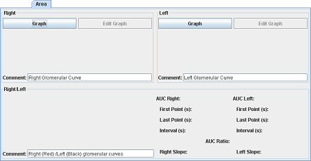
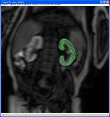
Draw a ROI on the dynamic stack with the ImageJ tools (freehand ROI is strongly recommended). This ROI must be limited to the parenchyma (cortex and medulla – excluding excretory system and fat). You can see an example on the following image. It may be necessary to register the images with use of a ROI during the 4 first minutes due to breathing motion of the kidney, especially in adults (use the registration tab).
Then, click on the “Graph” button to get the graph window. Be careful, the curve is normalized (see excretion tab).
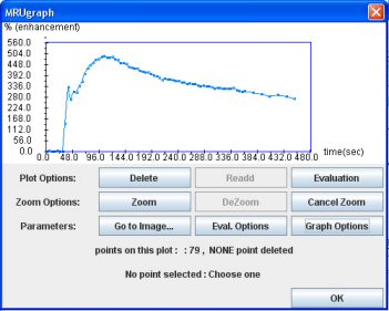
By clicking on “Graph Options”, you can focus on the relevant part of the curve: the ascending slope. This part begins at the minimum intensity point (P: Peak Trough) after the vascular peak (V) and ends with the maximum intensity point (G for glomerular point).
To compute the area under the curve:
- Click on “Evaluation”
- Then click on the first point of the ascending curve. By default the evaluation will correspond to a 60 second interval.
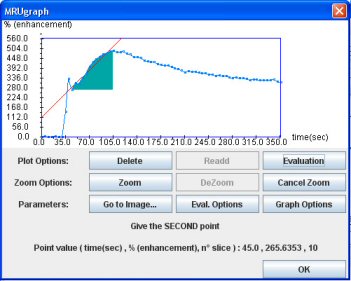
When you click on the OK button, the graph and the results appear on the main interface.
Repeat these actions for the other kidney (or pole) to get the area under the curve. Be careful to have the same time interval for the two curves. By clicking on “Evaluation” the same time interval as the first processed kidney will be proposed, by default. The times of the area under the curve can be modified as needed (see Notes).
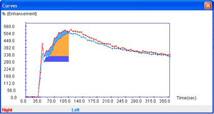
Once the areas under the curves have been determined for the two kidneys, the main interface computes the kidney function (only from the area values) and a third curve appears representing the intersection of the area in orange.
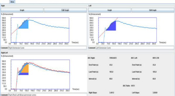
Double click on it to view it in a single window.
If you want to modify the graph or the parameters of the area, just click on the appropriate “Edit Graph” button or left double click. The “right double click” deletes the graph.
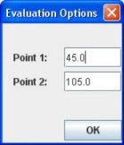
Note: You can specify manually the time points for the evaluation. Click on “Eval. Options” and specify your desired time points. Defaults values corresponding the controlateral kidney if already processed will be automatically applied. these values are the evaluation value for the other kidney/pole for this study).
Note: When you perform the evaluation, a red line appears. It represents the slope of the curve between the two evaluation points (Least squares approximation).
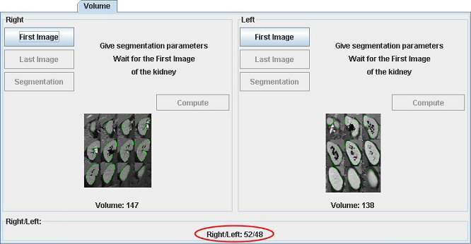
2) Volume tab: volume assessment
A stack of adjacent images is necessary to assess the renal volume (2D or 3D acquisition).
To compute the volume, the segmentation can be done:
- manually
- or semi-automatically (4). In the latter case, the algorithm used is based on the “Belief Functions Theory”. It consists on computing the mass of a pixel weighted by the information of its neighborhood in order to classify it in a region determine by the k-mean algorithm. Images need to be T1-weighted and fat-suppressed, and acquired at the end of the examination (bright urines) at the tubular phase after reinjection of 0.05 mmol/L of Gd-contrast medium. The goal is to have a satisfying contrast between kidney parenchyma (grey), urines (bright) and other organs and fat (dark).
4. Vivier PH, Dolores M, Gardin I, Zhang P, Petitjean C, Dacher JN. In vitro assessment of a 3D segmentation algorithm based on the belief functions theory in calculating renal volumes by MRI. AJR Am J Roentgenol 2008; 191:W127-134.
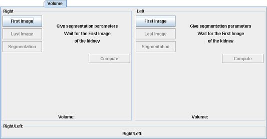
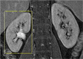
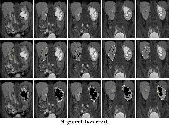
For semi-automatic segmentation: open the T1 weighted stack. Indicate the first, then the last image showing the studied kidney (pole). Draw a square ROI around it.
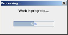
Then click on the segmentation button. A modal window appears showing the status of the work.
You can see on the stack the segmentation results. The ROI delimit the kidney and the cavities are black colored (fat too).
The volume tool appearance change too in order to allow the user to modify the segmentation results.
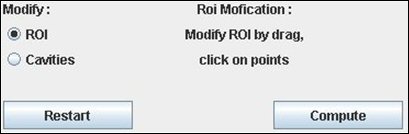
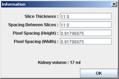
If automatic segmentation is appropriate, just “Compute”. Technical information (from DICOM headers) appears and needs control. If the information is correct, click “OK”, if not change it.
If changes are necessary, see below.
To switch between the ROI modification tool and the fat and cavities modification tool, you can either use the checkbox on the Volume manager or press the T key of your keyboard.
ROI modification:
1 – Move a point by select and drag (left mouse button)
2 – Move the ROI by select and drag (left mouse button)
3 – Delete a point by right clicking on it
4 – Delete a ROI by a double right click
5 – Create a new ROI by clicking on the left mouse button (point by point)
6 – To cut a ROI, click left on two points to be connected. Then, you can add intermediate points. Start from the last clicked point, and click left toward the first clicked one. Validate the result by a single right click.
For renal cavities and fat:
1 – Add Cavities/Fat: Press the left mouse button and use the cursor as a brush
2 – Remove Cavities/Fat: Press the right mouse button and use the cursor as a brush
3 – Remove all selected cavities: press the “R” key on your keyboard.
Note: By pressing the “escape” key, you can cancel the last modification.
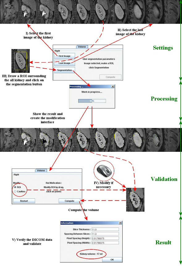
Volume (in ml) appears in the main interface as well. Image representing the segmented kidney appears (double click on it to enlarge it). To compare two kidneys (poles), you have to do the same action with the other one.
For manual segmentation, just unclick “automatic” and draw ROIs on each image displaying the kidney. Fat and cavities have to be excluded. See the previous “ROI modification” for exclusion of pixels and editing of the ROIs area.
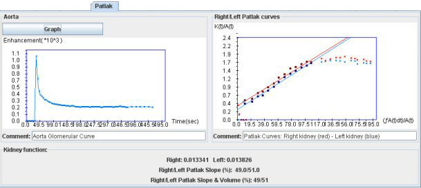
3) Rutland-Patlak plot
This step has to be performed after the “the area under the curves”. Indeed, the time interval used for the calculation of the slopes is the same as the one used for the area under the curves.
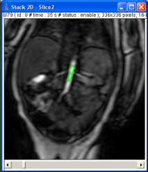
In the “Patlak tab”, first open a dynamic stack of images displaying the aorta (after having closed the previous stack). To avoid loading again images, you can spare some time by clicking on “View”, then on “3D Dynamic Window” (or the shortcut “ctrl+d”).
The first step is to draw a ROI on the aorta. Then, the aorta curve appears as well as the relevant part of the Patlak plot.
The split renal function determined from the ratio of the left and right (or lower-upper) slopes is provided. A volume-weighting is also yielded.
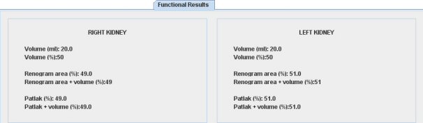
4) Using both area under the curve and volume (Area & Volume tab):
Split renal function is expressed in several ways: similar results between area under the curves and the Patlak plot provide some reliabity.
The results are expressed either with (“true results”) or without volume weighting (results in term of glomerular function per unit of volume parenchyma).
Interface configuration
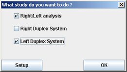
You can configure the interface in order to select only the different tab you need. When you start the plugin, before select the study you want to do, click “Setup”.
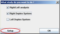
The following window appears. Check the tab you need and uncheck the others. This configuration is saved so when you will start again the plugin, you will not have to do this operation.
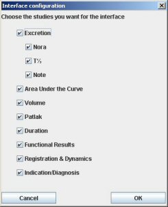
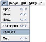
During the study you are able to add/remove the tab(s) by using the “Interface” item in the “File” menu. The modification is only available for this time and is not saved.
Note that only the tab presents are saved in the report.
The different working tools
I) Get the stack information:
To get the stack information, click on the “Info…” button in the Dicom Image Opener window. You can add information to this section, but only when you open a stack.
When you open a stack, you obtain the following window:
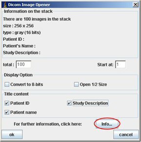
Click on the “Info…” button. You obtain a new window.
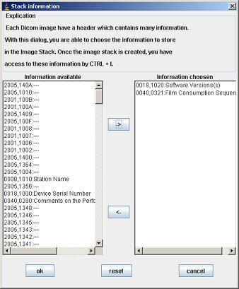
To add information, click on a line in the left section and then click on the “->” button. When you finish, click on “OK”.
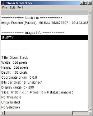
When you do “ctrl+i” on the stack, you get the following window:
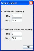
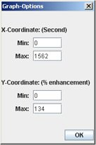
 II) Change the graph option:
It is possible to change the scale of the graph in the Graph window. You just have to click on the “Graph Options” button and then modify the value in the following window.
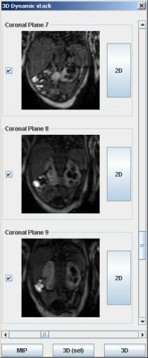
 III) Dynamic 3D stack:
To open a 3D dynamic stack, click on “Open Image/Stack”. Reach the file containing the dICOM images. If the file looks empty, choose “All files” in “Type of slices”.
Then click on one image to load all frames. A window displaying the different slices appears.
Different options are available:
- displaying different time points for all slices
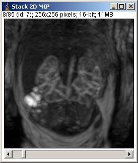
- clicking on “MIP”: it generates a dynamic stack of MIP (2D) images of selected slices (all slices are selected by default)
- clicking on “3D (sel)”: it opens a window with all selected slices at a chosen time point
- clicking on the “2D button”: it enables the dynamic analyzis by generating a 2D dynamic stack. You need first to choose the best slice displaying the desired kidney. You will be able to generate time-intensity curves by drawing ROIs (see “Excretion” and “Area under the curve” sections).
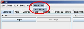
IV) The DICOM splitter:
To download an examination from a regular CD-ROM, click on “Sort exam”, then on “Sort Exam”.
Navigate to reach the "DICOM" file of the CD-ROM. Open it and click on "Save". Images downloading may take a few minutes depending on the size of the MR examination.
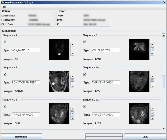
After having loaded the images a new window displaying the different sequences with their given name appears. You can store the images on your computer by clicking on “Hard Drive”. All sequences are selected by default and can be unselected.
V) The menu bar:
“File” menu:
– New: Restart with a blank interface
– Save: Save the study in order to re-open it in the future. The study is saved with the data (results and graph) and the different images added. The stack is not saved.
– Open: Open the previously saved study (save function). When you open the file, the program asks you to determine a workspace in order to work on this folder. Then all the things you will do and save will be added to this folder.
“?” menu:
– About: Get the version of the plug-in
Advice to avoid problems
- Have only one stack opened
- Open the stack with the plug-in (we keep information when opening it)
- Never associate different stacks in the same folder
- Respect the Dicom fields
- Follow the preceding instructions
- And read good articles :-)